

In this series of posts, I want to walk you through how to build a simple, persistent key-value store. We will be using an on-disk hashtable(also called external hashtable) to store the key-value mappings. In this post, I will explain hashtables briefly and an algorithm called linear hashing. In the next post, we’ll look at an implementation of linear hashing(written in Rust).
How would you store a hashtable on disk? This post describes a technique called linear hashing which can be used for this purpose. But before that let’s look at hashtables in general.
Hashtables primer
You might have seen in-memory implementations in an algorithms textbook or course that did something like the following. You create an array of fixed size n(the bucket array); when inserting a key-value pair (k,v), you take hash(k) mod n to get which slot in the array the pair will go into.
Because of something called the Birthday problem you expect there to be collisions– multiple keys being assigned to the same slot– even without having too many key-value pairs. To handle this, there are two schemes commonly presented:
The first idea is to have each entry in the array point to a linked list. When a key-value pair is assigned to a slot, it gets appended to the end of the linked list. A lookup would start at the head of the linked list and look at each node in the list until it finds the node with the key-value pair we’re looking for. This scheme is called separate chaining.
In the second scheme, slots in the array do not point to a linked list. They simply contain the key-value pair. Now, when a key-value pair is assigned to a slot and when the slot is occupied, we start scanning the array for a free slot. When doing a lookup, we would look at the slot the pair was assigned but notice that it’s not there. And start scanning the array to find it. This scheme is called open addressing.
Obviously I haven’t covered all the nuances of hashtable implementations here– there are corner cases I haven’t talked about and there are other schemes to deal with collision and hashtables. But there are plenty of fine resources that talk about those so we’ll move on to linear hashing.
Storing a hashtable to disk
Let’s now talk about how we would go about storing a hashtable in a file on disk. The technique I will describe, called linear hashing, is an adaptation of the first scheme(separate chaining) above. That means, our key-value pairs will be somehow stored in a linked list with array slots pointing to their corresponding linked lists(also called buckets).
However, unlike the in-memory version above, the nodes in the linked list won’t be storing a single pair. Files are organized in pages– each page is a block of bytes, usually 4KB in size; on Linux, you can run getconf PAGESIZE to see what it is on your system. While you can store values that span two blocks, say an 8-byte integer that starts at byte 4090 in the file and ending at byte 4097, the filesystem would have to read/write two pages to fulfill your request. Therefore, we will align a node in the linked list to a page. Each node will consist of multiple key-value pairs; once a page is full, we assign an overflow page linked to from the current page.
Both of the schemes described to deal with collision above are called static hashtable algorithms– the size of the bucket array stays the same[^1]. This can be a problem when we want to persist our hashtable to disk. In the separate chaining scheme, having a long chain of pages means that a lookup would us an I/O operation for each page. So, we want our linked lists to be really short.
Linear hashing
This is where linear hashing comes in. Linear hashing is a dynamic hashtable algorithm– the bucket array can grow as new key-value pairs are inserted. Keeping the chain of pages pointed at by the array slots short is the main goal of growing the bucket array. More specifically, it limits the average length of buckets(chain of linked list).
In linear hashing, when doing an insert, we start by looking at just the least significant bit(LSB) of the hash of the key. If it’s 0, it goes into the bucket 0 and if it’s 1, it goes into the bucket 1. We can keep inserting new items until the datastructure is utilized up to say 80%– that is, 80% of the storage allocated so far has been filled up.
When the threshold is crossed, we increment both number of bits and the number of buckets by 1. When we increment the number of bits, 0 and 1 become 00 and 01, respectively; for existing buckets, the representation changes to have two bits but their value is the same as before.
We add one bucket, 10. Note that incrementing number of bits by 1 doubles the number of addressable buckets, but we only increment the number of buckets by 1. Let’s now look at this newly added bucket– before we incremented the number of bits, all items whose hash’s LSB was 0 went to bucket 0(which is now bucket 00); some of those items may indeed have their two LSBs 00 but some of them may also have 10 as their two least LSBs. We want to move those to the 10 bucket. So, we iterate over the pairs in bucket 00 and re-insert each pair. This time, it’ll look at two bits in the hash and so the items will be inserted into either 00 or 10. Once we are done iterating we are done with the “growth” stage.
This is what our example hashtable looks like so far:

We calculate load factor as shown below:
num. of bits = 1
num. of buckets = 2
num. of items = 4

Load factor = num. of items / (num. of buckets * items per bucket)
            = 4  / (2 * 2) = 4/4
            = 1.0
Before, we pointed out that the number of addressable buckets doubled when we incremented number of bits ie. both 10 and 11 are representable with two bits. But we only added one bucket(10). Well, we’re looking at the last two bits of the hash, so what do we do if we see a hash with two LSBs 11? In that case, we need to simply ignore the MSB(1), and insert the pair into 01.
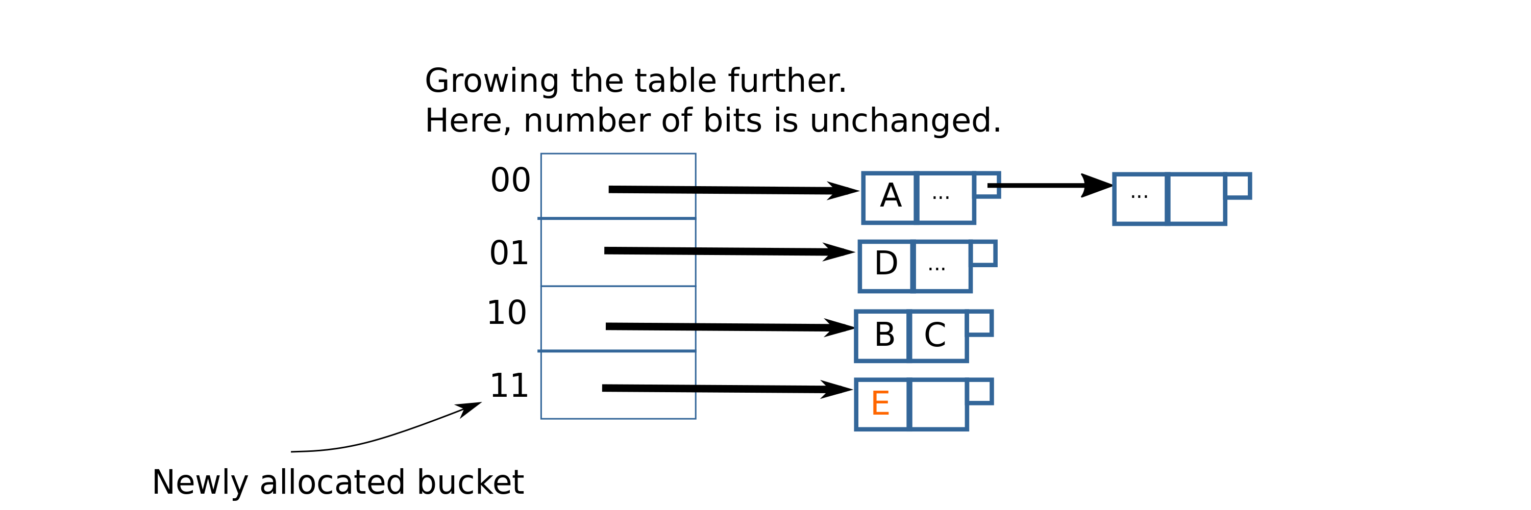
Let’s say that after inserting a few more items, the threshold is again exceeded. We need to grow the hashtable again. This time, however, we don’t increment the number of bits since there is already an unused address that is currently not in use(11). We just allocate space for the 11 bucket, and re-insert pairs in the 01 bucket.
After expanding the hashtable to allocate space for bucket 11, it will look like this:
Hashtable growth in linear hashing
Growing the hashtable is what makes linear hashing a dynamic hashtable algorithm. And so, it’s important to understand how the hashtable grows. As we saw, first the 10 bucket is added causing the 00 bucket to be split(ie. bucket 00’s items were re-distributed between 00 and 10).
Later on, when the hashtable’s load factor crossed the threshold again, bucket 11 was added. This time, bucket 01 was split. As more items are inserted, the next buckets to be split will be 000(100 added), 001(101 added), and so on.
There are two important characteristics to how hashtables grow under the linear hashing algorithm. First, the hashtable grows linearly– an insert will cause one bucket to split[^2]. This gives us some assurance that insert performance doesn’t degrade. Second, all buckets are split eventually. This property will ensure that the linked lists pointed to by the bucket array don’t get too long.
One last thing worth pointing out is that the order in which buckets get split is deterministic, in linear order. Usually, the bucket split is different than the one to which a key-value pair was just inserted.
Conclusion
That’s it for now. Hopefully, you have some intuition for why we use linear hashing– that is, to avoid accessing multiple pages when looking up a key in the hashtable. And also why linear hashing works. In the next post we’ll look at a Rust implementation of linear hashing. In case you don’t want to wait, you can check out the implementation on Github.
Update: Part two of this series is now up.
Update: There’s some interesting discussion in this post’s Reddit thread
[^1]: Both of these schemes can support a re-hash operation, however
 that can be time-consuming. And the hashtable will be unusable
 during the rehash.
[^2]: Proof: Let $r$ be the number of records, $n$ be the number of
buckets, $b$ be the number of records per bucket and $t$ be the
threshold. We know that $\frac{r}{bn} < t$. When we insert a new
record, the load exceeds threshold: $\frac{r+1}{n} > bt$.  After
splitting a bucket we have, $$\text{load factor} =
\frac{r+1}{n+1}$$ We want to show that after splitting once, this
new *load factor* < t. Since $r < btn$, $r + 1 < btn + 1$. Then,
since $b > 1$ and $0 < t \leq 1$, we know that $bt > 1$. So $r+1 <
btn + bt$, so, $r + 1 < bt(n + 1)$. Hence, $$\frac{r+1}{n+1} < bt$$
which is equivalent to $$\text{load factor} < t$$ Thus, we know
that we will only have to split once bucket per insert.